Demonstration of `hii_region_model`

Bayesian kinematic distance calculator.

Trey Wenger, 2025

[1]:

import pickle
import numpy as np
from scipy.stats import multivariate_normal
import pymc as pm
import arviz as az
import pandas as pd
import matplotlib.pyplot as plt

from physiokinematic.hii_region_model import hii_region_model

[2]:

# Load Reid et al. (2019) rotation curve parameters
with open("../../../data/reid19_params.pkl", "rb") as f:
    reid19_params = pickle.load(f)
print(reid19_params.keys())

samples = reid19_params['full'].resample(1_000)

# R0, Usun, Vsun, Wsun, a2, a3
samples = samples[np.array([0,1,2,3,6,7]), :]

reid19_fit = multivariate_normal.fit(samples.T)

dict_keys(['R0', 'Usun', 'Vsun', 'Wsun', 'Upec', 'Vpec', 'a2', 'a3', 'full'])

/tmp/ipykernel_331801/3720529096.py:3: DeprecationWarning: Please import `gaussian_kde` from the `scipy.stats` namespace; the `scipy.stats.kde` namespace is deprecated and will be removed in SciPy 2.0.0.
  reid19_params = pickle.load(f)

[3]:

hii_data = pd.read_csv("../../../data/hii_data.csv")
data = hii_data.iloc[550].copy()
data

[3]:

gname                   G035.126-00.755
glong                            35.126
glat                          -0.754265
radius                          169.392
vlsr                               34.5
e_vlsr                              0.1
line                              29.48
e_line                            0.204
line_unit                      mJy/beam
beam_area                   6893.719776
line_freq                        8000.0
fwhm                               19.7
e_fwhm                              0.2
te                                  NaN
e_te                              500.0
source                     WISE Catalog
author          Anderson et al. (2015b)
telescope                           GBT
kdar                                  N
Rgal                           6.567508
near                           2.055998
far                           11.270497
tangent                        6.676467
vlsr_tangent                  96.219351
plx                                 NaN
dist_author                         NaN
te_priority                           0
Name: 550, dtype: object

[4]:

model = hii_region_model(
    data, # HII region data
    reid19_fit[0], # Prior mean on rotation curve parameters
    reid19_fit[1], # Prior covariance on rotation curve parameters
    prior_Rgal = 5.0, # Prior width on Galactocentric radius (kpc)
    prior_te_offset = [4500.0, 200.0], # Prior mean and width on electron temperature gradient offset (K)
    prior_te_slope = [360.0, 25.0], # Prior mean and width on elecron temperature gradient slope (K/kpc)
    prior_log10_q = [47.0, 2.0], # Prior mean and width on log10 ionizing photon rate (s-1)
    prior_log10_ne = [1.0, 2.0], # Prior mean and width on log10 electron density (cm-3)
    prior_kdar = [0.5, 0.5], # Prior shape for kinematic distance ambiguity resolution
    log10_radius_sigma = 0.1, # Apparent radius likelihood width
    log10_line_sigma = 0.2, # Line brightness likelihood width
    vlsr_sigma = 10.0, # Assumed LSR velocity systematic uncertainty (km/s)
    te_sigma = 500.0, # Assumed electron temperature systematic uncertainty (K)
)

[5]:

model

[5]:

$$ \begin{array}{rcl} \text{rotcurve} &\sim & \operatorname{MultivariateNormal}(f(),~\text{<constant>})\\\text{Rgal_norm} &\sim & \operatorname{Gamma}(0.5,~f())\\\text{te_offset_norm} &\sim & \operatorname{Normal}(0,~1)\\\text{te_slope_norm} &\sim & \operatorname{Normal}(0,~1)\\\text{te_norm} &\sim & \operatorname{Normal}(0,~1)\\\text{kdar_w} &\sim & \operatorname{Categorical}(\text{<constant>})\\\text{log10_q_norm} &\sim & \operatorname{Normal}(0,~1)\\\text{log10_ne_norm} &\sim & \operatorname{Normal}(0,~1)\\\text{Rgal} &\sim & \operatorname{Deterministic}(f(\text{Rgal_norm},~\text{rotcurve}))\\\text{te_offset} &\sim & \operatorname{Deterministic}(f(\text{te_offset_norm}))\\\text{te_slope} &\sim & \operatorname{Deterministic}(f(\text{te_slope_norm}))\\\text{te} &\sim & \operatorname{Deterministic}(f(\text{te_norm},~\text{te_offset_norm},~\text{te_slope_norm},~\text{Rgal_norm},~\text{rotcurve}))\\\text{distance} &\sim & \operatorname{Deterministic}(f(\text{rotcurve},~\text{Rgal_norm}))\\\text{abs_distance} &\sim & \operatorname{Deterministic}(f(\text{rotcurve},~\text{Rgal_norm}))\\\text{log10_q} &\sim & \operatorname{Deterministic}(f(\text{log10_q_norm}))\\\text{log10_ne} &\sim & \operatorname{Deterministic}(f(\text{log10_ne_norm}))\\\text{log10_Rs} &\sim & \operatorname{Deterministic}(f(\text{log10_q_norm},~\text{log10_ne_norm}))\\\text{log10_em} &\sim & \operatorname{Deterministic}(f(\text{log10_ne_norm},~\text{log10_q_norm}))\\\text{log10_radius_mu} &\sim & \operatorname{Deterministic}(f(\text{log10_q_norm},~\text{log10_ne_norm},~\text{rotcurve},~\text{Rgal_norm}))\\\text{log10_tau_line} &\sim & \operatorname{Deterministic}(f(\text{log10_ne_norm},~\text{te_norm},~\text{log10_q_norm},~\text{te_offset_norm},~\text{te_slope_norm},~\text{Rgal_norm},~\text{rotcurve}))\\\text{log10_line_mu} &\sim & \operatorname{Deterministic}(f(\text{te_norm},~\text{te_offset_norm},~\text{te_slope_norm},~\text{Rgal_norm},~\text{rotcurve},~\text{log10_ne_norm},~\text{log10_q_norm}))\\\text{vlsr_obs} &\sim & \operatorname{Normal}(f(\text{rotcurve},~\text{Rgal_norm}),~f())\\\text{log10_radius_obs} &\sim & \operatorname{Normal}(f(\text{kdar_w},~\text{log10_q_norm},~\text{log10_ne_norm},~\text{rotcurve},~\text{Rgal_norm}),~0.1)\\\text{log10_line_obs} &\sim & \operatorname{Normal}(f(\text{kdar_w},~\text{te_norm},~\text{te_offset_norm},~\text{te_slope_norm},~\text{Rgal_norm},~\text{rotcurve},~\text{log10_q_norm},~\text{log10_ne_norm}),~0.2) \end{array} $$

[6]:

# sample prior predictive
with model:
    prior = pm.sample_prior_predictive(1_000)

Sampling: [Rgal_norm, kdar_w, log10_line_obs, log10_ne_norm, log10_q_norm, log10_radius_obs, rotcurve, te_norm, te_offset_norm, te_slope_norm, vlsr_obs]

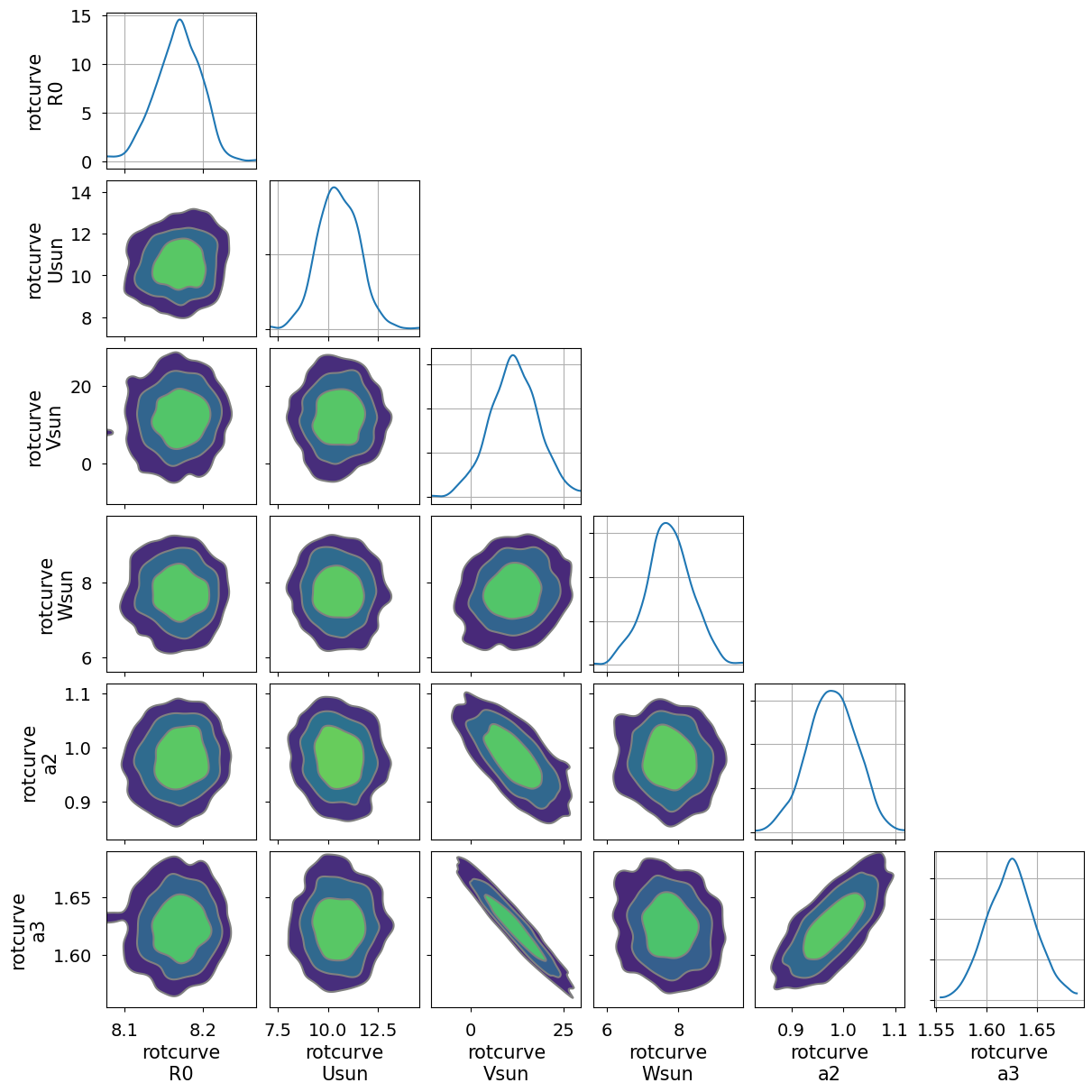
[7]:

# plot prior samples
_ = pm.plot_pair(prior.prior["rotcurve"], marginals=True, figsize=(12, 12), kind='kde', backend_kwargs={"layout": "constrained"})

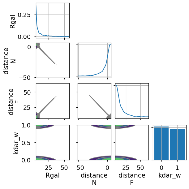
../_images/notebooks_hii_region_model_7_0.png

[8]:

# plot prior samples
_ = pm.plot_pair(prior.prior, marginals=True, figsize=(6, 6), kind='kde', backend_kwargs={"layout": "constrained"}, var_names=["Rgal", "distance", "kdar_w"])

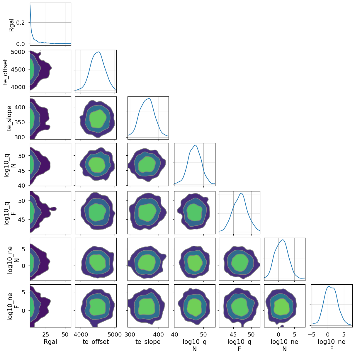
../_images/notebooks_hii_region_model_8_0.png

[9]:

# plot prior samples
_ = pm.plot_pair(prior.prior, marginals=True, figsize=(12, 12), kind='kde', backend_kwargs={"layout": "constrained"}, var_names=["Rgal", "te_offset", "te_slope", "log10_q", "log10_ne"])

../_images/notebooks_hii_region_model_9_0.png

[10]:

# The model is multi-modal, so we sample with SMC
with model:
    trace = pm.sample_smc()

Initializing SMC sampler...
Sampling 12 chains in 12 jobs

 |████████████████████████████████████████| 100.00% [100/100 00:00<?  Stage: 5 Beta: 1.000]

/home/twenger/miniforge3/envs/physiokinematic/lib/python3.12/site-packages/arviz/data/base.py:272: UserWarning: More chains (12) than draws (6). Passed array should have shape (chains, draws, *shape)
  warnings.warn(

[11]:

az.summary(trace, hdi_prob=0.68, var_names=["rotcurve", "Rgal", "distance", "kdar_w", "te_offset", "te_slope", "te", "log10_q", "log10_ne", "log10_Rs", "log10_em"])

[11]:

	mean	sd	hdi_16%	hdi_84%	mcse_mean	mcse_sd	ess_bulk	ess_tail	r_hat
rotcurve[R0]	8.169	0.027	8.142	8.195	0.000	0.000	4827.0	6154.0	1.00
rotcurve[Usun]	10.472	1.000	9.516	11.500	0.014	0.010	5528.0	5232.0	1.00
rotcurve[Vsun]	12.239	6.206	6.272	18.415	0.084	0.063	5542.0	6083.0	1.00
rotcurve[Wsun]	7.729	0.603	7.141	8.346	0.009	0.006	4877.0	4900.0	1.00
rotcurve[a2]	0.977	0.044	0.937	1.024	0.001	0.000	5032.0	5156.0	1.00
rotcurve[a3]	1.622	0.023	1.600	1.645	0.000	0.000	5711.0	4945.0	1.00
Rgal	6.575	0.443	6.133	6.992	0.005	0.003	7061.0	9005.0	1.00
distance[N]	2.106	0.640	1.521	2.763	0.008	0.005	7007.0	9323.0	1.00
distance[F]	11.256	0.639	10.621	11.860	0.008	0.005	7058.0	9015.0	1.00
kdar_w	0.666	0.471	0.000	1.000	0.008	0.003	3457.0	3457.0	1.01
te_offset	4497.532	192.992	4300.229	4687.081	2.448	1.692	6249.0	6044.0	1.00
te_slope	360.109	24.991	335.782	384.921	0.344	0.287	5285.0	5046.0	1.00
te	6861.651	567.517	6314.482	7427.825	7.463	5.651	5760.0	3964.0	1.00
log10_q[N]	46.355	1.667	44.691	47.650	0.023	0.016	5415.0	5771.0	1.00
log10_q[F]	46.789	0.908	46.280	47.115	0.020	0.027	2790.0	1480.0	1.01
log10_ne[N]	1.320	1.531	-0.012	2.537	0.020	0.018	6291.0	5386.0	1.01
log10_ne[F]	1.445	0.980	1.210	1.986	0.025	0.036	2492.0	591.0	1.00
log10_Rs[N]	0.718	1.219	-0.336	1.751	0.016	0.013	6227.0	5621.0	1.00
log10_Rs[F]	0.779	0.699	0.456	0.887	0.017	0.025	2413.0	674.0	1.01
log10_em[N]	3.659	2.051	1.671	5.156	0.026	0.025	6306.0	4964.0	1.01
log10_em[F]	3.970	1.363	3.515	4.725	0.034	0.050	2467.0	1300.0	1.01

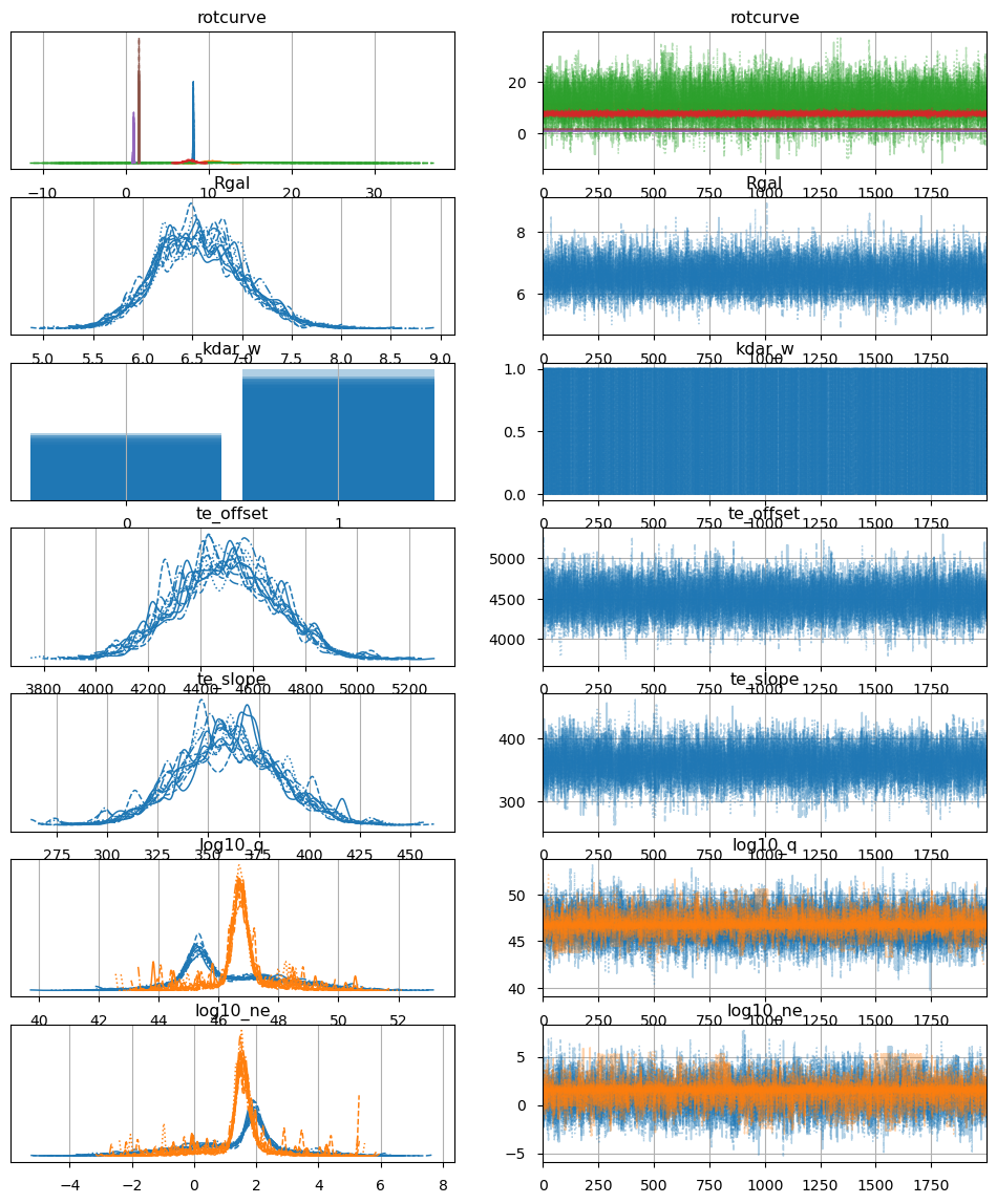
[12]:

_ = pm.plot_trace(trace.posterior, var_names=["rotcurve", "Rgal", "kdar_w", "te_offset", "te_slope", "log10_q", "log10_ne"])

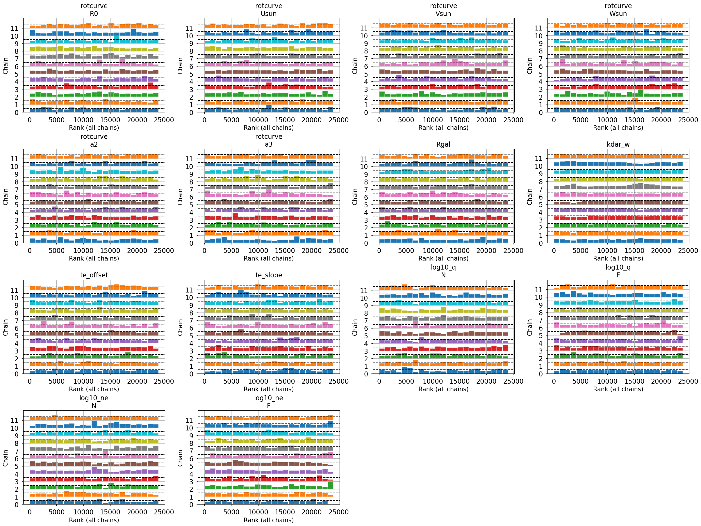
../_images/notebooks_hii_region_model_12_0.png

[13]:

_ = pm.plot_rank(trace.posterior, var_names=["rotcurve", "Rgal", "kdar_w", "te_offset", "te_slope", "log10_q", "log10_ne"], figsize=(24, 18), backend_kwargs={"layout": "constrained"})

../_images/notebooks_hii_region_model_13_0.png

[14]:

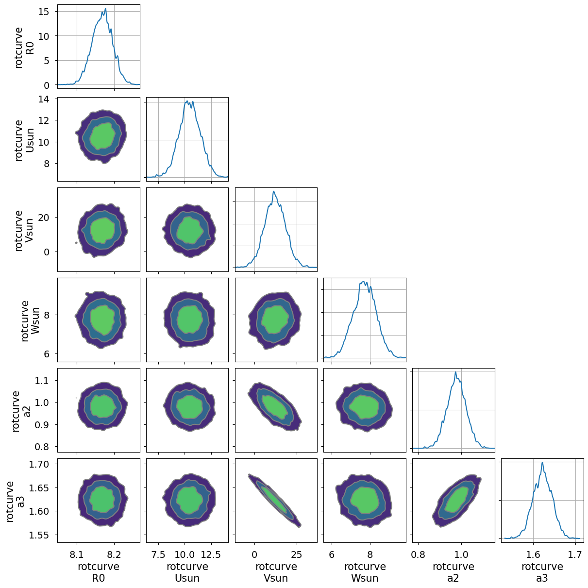
# plot posterior samples
_ = pm.plot_pair(trace.posterior["rotcurve"], marginals=True, figsize=(12, 12), kind='kde', backend_kwargs={"layout": "constrained"})

../_images/notebooks_hii_region_model_14_0.png

[15]:

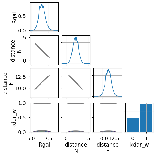
# plot posterior samples
_ = pm.plot_pair(trace.posterior, marginals=True, figsize=(6, 6), kind='kde', backend_kwargs={"layout": "constrained"}, var_names=["Rgal", "distance", "kdar_w"])

../_images/notebooks_hii_region_model_15_0.png

[16]:

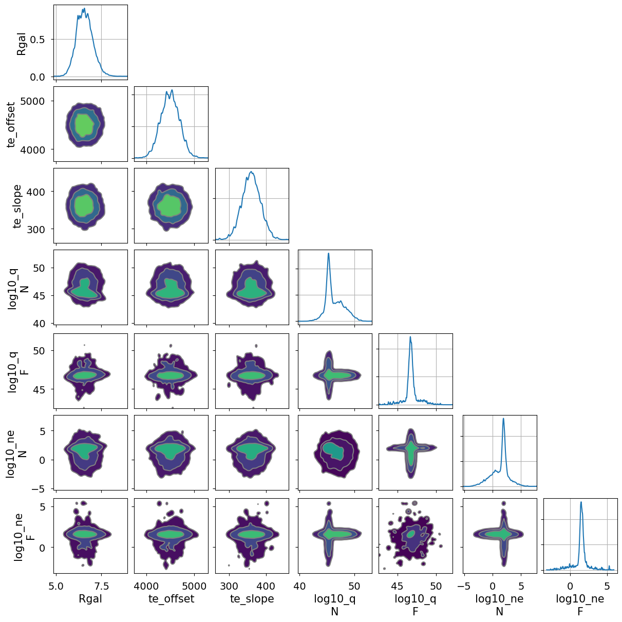
# plot posterior samples
_ = pm.plot_pair(trace.posterior, marginals=True, figsize=(12, 12), kind='kde', backend_kwargs={"layout": "constrained"}, var_names=["Rgal", "te_offset", "te_slope", "log10_q", "log10_ne"])

../_images/notebooks_hii_region_model_16_0.png

[17]:

# sample posterior predictive
with model:
    posterior = pm.sample_posterior_predictive(trace.sel(draw=slice(None, None, 1)))

Sampling: [log10_line_obs, log10_radius_obs, vlsr_obs]

100.00% [24000/24000 00:01<00:00]

[18]:

# drop samples with distance <= 0.0
bad_distance = trace.posterior["distance"] <= 0.0

result = {}

# Hyperparameters & distance-independent parameters
params = ["te_offset", "te_slope", "Rgal", "te"]
for param in params:
    if param not in trace.posterior:
        continue
    post = trace.posterior[param].data.flatten()
    result[f"{param}_mean"] = np.mean(post)
    result[f"{param}_std"] = np.std(post)
    result[f"{param}_median"] = np.median(post)
    hdi = az.hdi(post, hdi_prob=0.90)
    result[f"{param}_hdi5"] = hdi[0]
    result[f"{param}_hdi95"] = hdi[1]

# Distance-dependent parameters
params = [
    "distance",
    "log10_q",
    "log10_ne",
    "log10_Rs",
    "log10_em",
    "log10_tau_line",
    "log10_radius_mu",
    "log10_line_mu",
]
for param in params:
    posterior_N = trace.posterior[param].sel(kdar="N").data[
        (trace.posterior["kdar_w"] == 0) * (~bad_distance.sel(kdar="N"))
    ]
    posterior_F = trace.posterior[param].sel(kdar="F").data[
        (trace.posterior["kdar_w"] == 1) * (~bad_distance.sel(kdar="F"))
    ]
    posterior_T = np.concatenate([posterior_N, posterior_F])
    for kdar, post in zip(["N", "F", "T"], [posterior_N, posterior_F, posterior_T]):
        if len(post) < 5:
            continue
        result[f"{param}_{kdar}_mean"] = np.mean(post)
        result[f"{param}_{kdar}_std"] = np.std(post)
        result[f"{param}_{kdar}_median"] = np.median(post)
        hdi = az.hdi(post, hdi_prob=0.90)
        result[f"{param}_{kdar}_hdi5"] = hdi[0]
        result[f"{param}_{kdar}_hdi95"] = hdi[1]

    result[f"{param}_samples"] = posterior_T

# KDAR weight
result["kdar_w"] = len(posterior_F)/len(posterior_T)

# Observed parameters
params = [
    "vlsr_obs",
    "log10_radius_obs",
    "log10_line_obs",
]
for param in params:
    post = posterior.posterior_predictive[param].data.flatten()
    result[f"{param}_mean"] = np.mean(post)
    result[f"{param}_std"] = np.std(post)
    result[f"{param}_median"] = np.median(post)
    hdi = az.hdi(post, hdi_prob=0.90)
    result[f"{param}_hdi5"] = hdi[0]
    result[f"{param}_hdi95"] = hdi[1]
    result[f"{param}_samples"] = post

[19]:

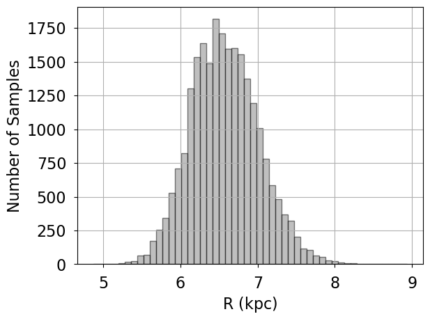
fig, ax = plt.subplots()
ax.hist(trace.posterior["Rgal"].data.flatten(), bins=50, color="gray", edgecolor="k", alpha=0.5)
ax.set_ylabel("Number of Samples")
ax.set_xlabel("$R$ (kpc)")

[19]:

Text(0.5, 0, '$R$ (kpc)')

../_images/notebooks_hii_region_model_19_1.png

[20]:

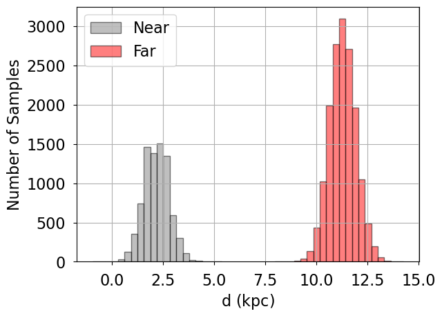
fig, ax = plt.subplots()
bins=20
ax.hist(trace.posterior["distance"].sel(kdar='N').data.flatten(), weights=(1-trace.posterior["kdar_w"].data.flatten()), bins=bins, color="gray", edgecolor="k", alpha=0.5, label="Near")
ax.hist(trace.posterior["distance"].sel(kdar='F').data.flatten(), weights=trace.posterior["kdar_w"].data.flatten(), bins=bins, color="red", edgecolor="k", alpha=0.5, label="Far")
ax.set_ylabel("Number of Samples")
ax.set_xlabel("$d$ (kpc)")
ax.legend(loc="best")

[20]:

<matplotlib.legend.Legend at 0x7bcef9072c60>

../_images/notebooks_hii_region_model_20_1.png

[21]:

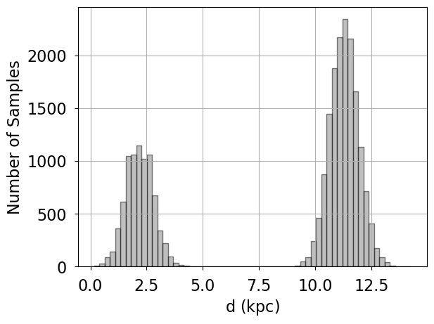
fig, ax = plt.subplots()
bins=60
ax.hist(result["distance_samples"], bins=bins, color="gray", edgecolor="k", alpha=0.5)
ax.set_ylabel("Number of Samples")
ax.set_xlabel("$d$ (kpc)")

[21]:

Text(0.5, 0, '$d$ (kpc)')

../_images/notebooks_hii_region_model_21_1.png

[22]:

print(result["kdar_w"])

0.6665555462955246

[23]:

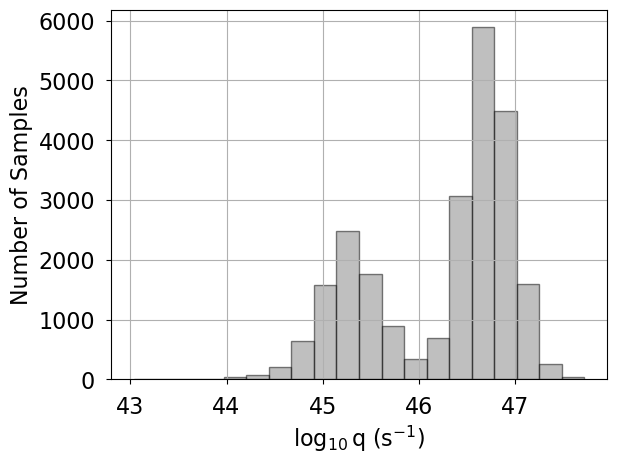
fig, ax = plt.subplots()
bins=20
ax.hist(result["log10_q_samples"], bins=bins, color="gray", edgecolor="k", alpha=0.5)
ax.set_ylabel("Number of Samples")
ax.set_xlabel(r"$\log_{10} q$ (s$^{-1}$)")

[23]:

Text(0.5, 0, '$\\log_{10} q$ (s$^{-1}$)')

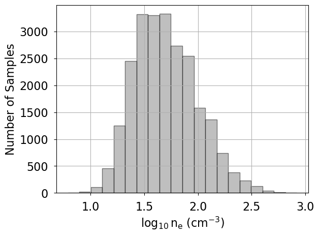
../_images/notebooks_hii_region_model_23_1.png

[24]:

fig, ax = plt.subplots()
bins=20
ax.hist(result["log10_ne_samples"], bins=bins, color="gray", edgecolor="k", alpha=0.5)
ax.set_ylabel("Number of Samples")
ax.set_xlabel(r"$\log_{10} n_e$ (cm$^{-3}$)")

[24]:

Text(0.5, 0, '$\\log_{10} n_e$ (cm$^{-3}$)')

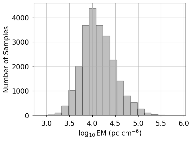
../_images/notebooks_hii_region_model_24_1.png

[25]:

fig, ax = plt.subplots()
bins=20
ax.hist(result["log10_em_samples"], bins=bins, color="gray", edgecolor="k", alpha=0.5)
ax.set_ylabel("Number of Samples")
ax.set_xlabel(r"$\log_{10} EM$ (pc cm$^{-6}$)")

[25]:

Text(0.5, 0, '$\\log_{10} EM$ (pc cm$^{-6}$)')

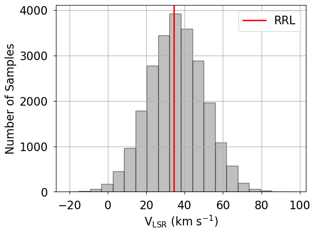
../_images/notebooks_hii_region_model_25_1.png

[26]:

# plot posterior predictive samples
fig, ax = plt.subplots()
bins=20
ax.hist(result["vlsr_obs_samples"], bins=bins, color="gray", edgecolor="k", alpha=0.5)
ax.axvline(data["vlsr"], color="r", lw=2, label="RRL")
ax.set_ylabel("Number of Samples")
ax.set_xlabel(r"$V_{\rm LSR}$ (km s$^{-1}$)")
ax.legend(loc="best")

[26]:

<matplotlib.legend.Legend at 0x7bcefbf9e3c0>

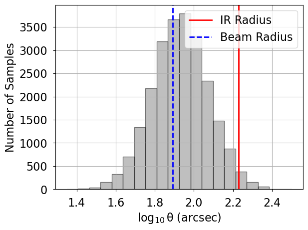
../_images/notebooks_hii_region_model_26_1.png

[27]:

# plot posterior predictive samples
fig, ax = plt.subplots()
bins=20
ax.hist(result["log10_radius_obs_samples"], bins=bins, color="gray", edgecolor="k", alpha=0.5)
ax.axvline(np.log10(data["radius"]), color="r", lw=2, label="IR Radius")
beam_radius = np.sqrt(data["beam_area"]*4.0*np.log(2.0)/np.pi)
ax.axvline(np.log10(beam_radius), color="b", lw=2, ls="--", label="Beam Radius")
ax.set_ylabel("Number of Samples")
ax.set_xlabel(r"$\log_{10} \theta$ (arcsec)")
ax.legend(loc="best")

[27]:

<matplotlib.legend.Legend at 0x7bcefc3e7050>

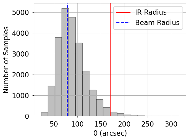
../_images/notebooks_hii_region_model_27_1.png

[28]:

# plot posterior predictive samples
fig, ax = plt.subplots()
bins=20
ax.hist(10.0**result["log10_radius_obs_samples"], bins=bins, color="gray", edgecolor="k", alpha=0.5)
ax.axvline(data["radius"], color="r", lw=2, label="IR Radius")
beam_radius = np.sqrt(data["beam_area"]*4.0*np.log(2.0)/np.pi)
ax.axvline(beam_radius, color="b", lw=2, ls="--", label="Beam Radius")
ax.set_ylabel("Number of Samples")
ax.set_xlabel(r"$\theta$ (arcsec)")
ax.legend(loc="best")

[28]:

<matplotlib.legend.Legend at 0x7bcefc3e63c0>

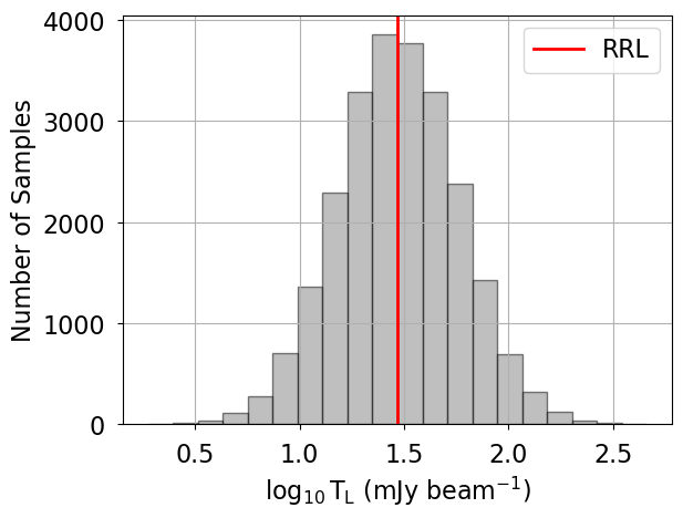
../_images/notebooks_hii_region_model_28_1.png

[29]:

# plot posterior predictive samples
fig, ax = plt.subplots()
bins=20
ax.hist(result["log10_line_obs_samples"], bins=bins, color="gray", edgecolor="k", alpha=0.5)
ax.axvline(np.log10(data["line"]), color="r", lw=2, label="RRL")
ax.set_ylabel("Number of Samples")
ax.set_xlabel(r"$\log_{10} T_L$ (mJy beam$^{-1}$)")
ax.legend(loc="best")

[29]:

<matplotlib.legend.Legend at 0x7bcefc0a63c0>

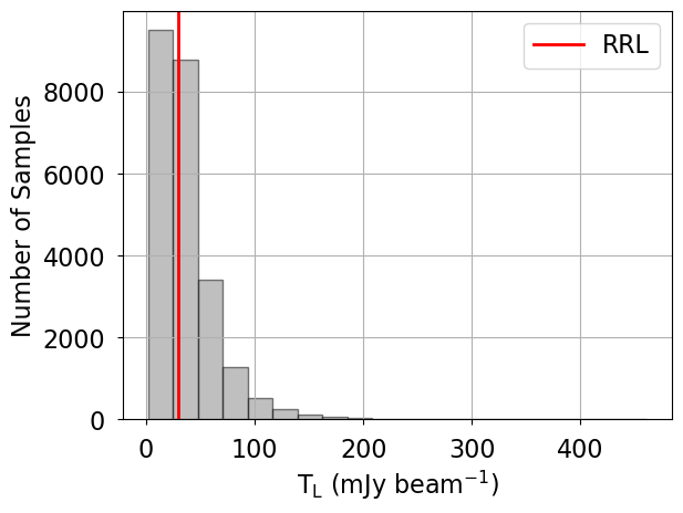
../_images/notebooks_hii_region_model_29_1.png

[30]:

# plot posterior predictive samples
fig, ax = plt.subplots()
bins=20
ax.hist(10.0**result["log10_line_obs_samples"], bins=bins, color="gray", edgecolor="k", alpha=0.5)
ax.axvline(data["line"], color="r", lw=2, label="RRL")
ax.set_ylabel("Number of Samples")
ax.set_xlabel(r"$T_L$ (mJy beam$^{-1}$)")
ax.legend(loc="best")

[30]:

<matplotlib.legend.Legend at 0x7bcefbee88c0>

../_images/notebooks_hii_region_model_30_1.png

[ ]:

Demonstration of hii_region_model

Demonstration of `hii_region_model`